Orion: A Fully Homomorphic Encryption Framework for Deep Learning
- Written by Austin Ebel, Karthik Garimella, Brandon Reagen (New York University)
- Based on https://arxiv.org/pdf/2311.03470 (ASPLOS 2025)
TL;DR: Orion is a framework that compiles PyTorch neural network models into efficient CKKS FHE programs for encrypted inference. Orion automatically handles low-level FHE details such as data packing, bootstrap placement, and precision management. Orion is open-sourced at: https://github.com/baahl-nyu/orion.
1. Introduction
The CKKS FHE scheme enables cryptographically secure outsourced computing, which has broad implications for areas such as health or finance. However, writing FHE programs, especially FHE neural networks, remains a challenge given the low-level primitives that CKKS exposes: addition, multiplication, and rotation of encrypted vectors. Furthermore, auxiliary FHE operations that are necessary for deep computations (such as bootstrapping and scale management) only make this harder.
A user of FHE might ask: How and when should bootstraps be placed during inference? What FHE algorithm should be used for computing convolutions? How can we approximate non-linear activations? In this blog, we introduce our framework Orion, which handles each of these issues automatically, making it easier to write FHE neural network programs. The figure below describes three key aspects we had in mind when building Orion.

First, we automatically handle FHE packing in order to leverage fast CKKS linear transformation algorithms. Our packing strategy ensures that each linear layer consumes only one multiplicative level regardless of the linear layer configuration. Second, we entirely automate both bootstrap and scale management, which enables Orion to run deep neural networks such as ResNet-50 while still maintaining precision. Finally, we wanted Orion to be accessible; writing FHE neural networks in Orion requires only knowledge of PyTorch.
Below, we’ll cover the details of our convolution algorithm and bootstrap placement strategy.
2. Efficient Linear Transform Algorithms
Linear transformations are a core building block in neural networks, from convolutional neural networks (convolutions, average pooling, and final head layers) to modern-day transformer architectures (QKV projections, feed-forward MLPs, and even RoPE). Under CKKS, it helps to think about linear transforms in terms of three constraints: how well we use ciphertext slots, how many multiplicative levels we consume, and how many expensive homomorphic operations we require (in particular, key-switches induced by ciphertext rotations).
As a concrete example, consider outsourced neural inference where we want to compute a matrix–vector product between a plaintext weight matrix and an encrypted ciphertext vector. Since the weight matrix is unencrypted, it can be packed into CKKS plaintext vectors in different ways, and that packing choice largely determines how many rotations and levels we pay for.
A natural first attempt is to pack each row of the matrix into a CKKS vector and compute a dot product against the ciphertext. In practice, row-based packing tends to be a poor fit for CKKS: it requires padding dimensions to powers of two, it computes dot products within ciphertexts (often leading to low slot utilization), and it typically consumes extra multiplicative depth to consolidate partial sums. It also scales poorly in rotations for dense matrix–vector products.

Orion instead targets diagonal-based matrix–vector product algorithms in which the diagonals of the unencrypted matrix are packed into CKKS vectors. These algorithms have been well-optimized by the cryptographic community, and they align well with how CKKS bootstrapping itself is implemented (which relies on large linear transforms). Rather than computing dot products within intermediate ciphertexts, diagonal-based approaches compute dot products across ciphertexts and then aggregate them into a single packed ciphertext output.
A standard way to reduce the rotation count further is the baby-step giant-step (BSGS) strategy. Informally, BSGS reuses ciphertext rotations by reorganizing which shifts happen on ciphertexts and which shifts can be absorbed into plaintext preprocessing of packed diagonals. This reduces rotation counts from $O(n)$ down to $O(\sqrt{n})$ while still consuming only one multiplicative level.

In Orion, we combine BSGS with low-level cryptographic optimizations (in particular, double hoisting) to reduce the amortized cost per rotation. Once we treat “fast matrix–vector products” as a first-class compiler target, we can build higher-level neural network layers on top of a kernel that is both level-efficient (one level per MV) and rotation-efficient (BSGS + hoisting).
3. Convolutions as Matrix-Vector Products
Now that we have a blueprint for fast matrix-vector products, a natural question is: can we apply it to convolutions? If so, then the same principles would extend to the much wider class of convolutional neural nets.
The standard approach for this is known as the Toeplitz formulation. Here, the input image is flattened into a vector and the kernel expands into a matrix. Each row of this Toeplitz matrix corresponds to one filter multiplication with the input image as it slides over all of its positions.
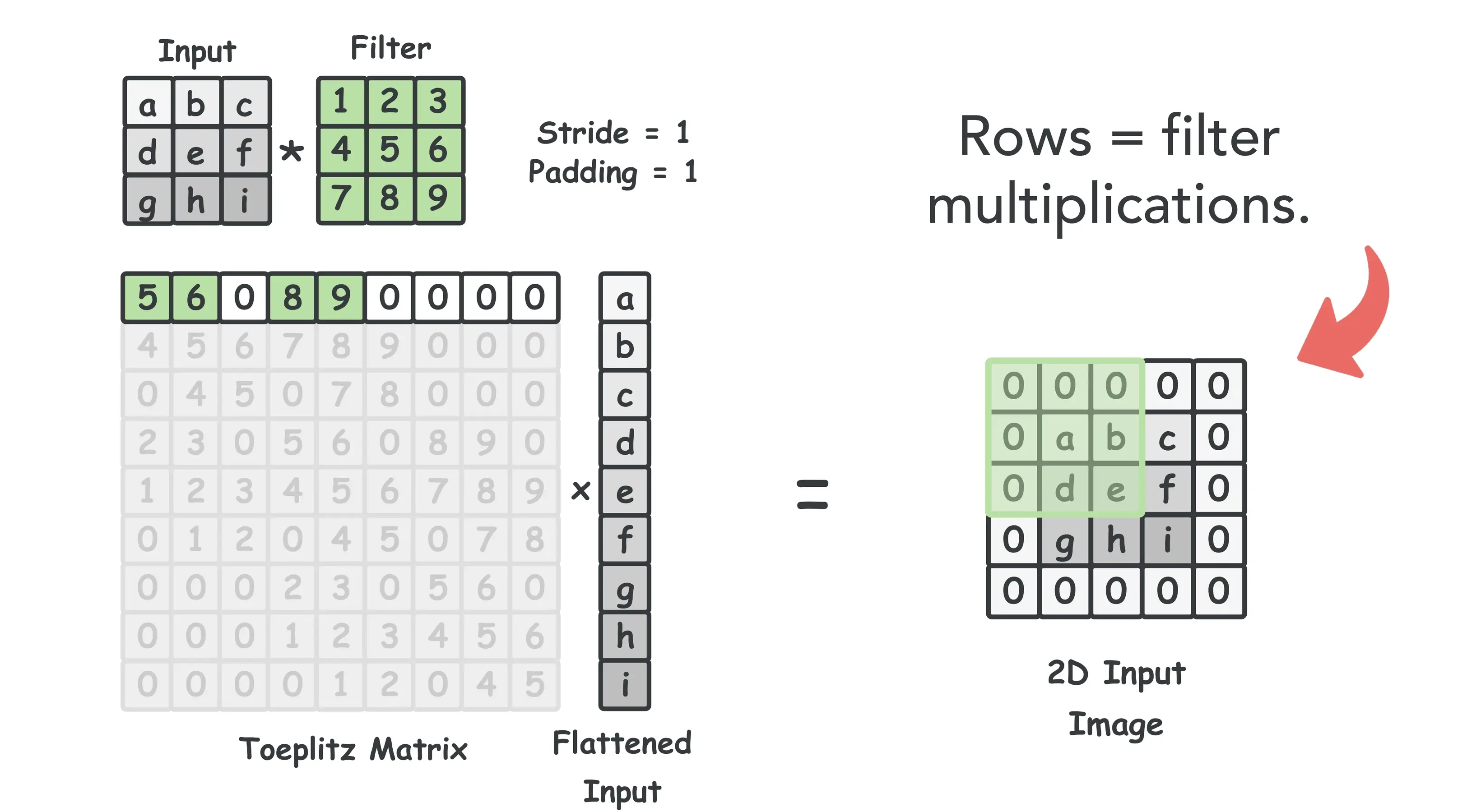
The animation in Figure 4 shows this for single-input single-output (SISO) convolutions, although the approach naturally extends to multi-input, multi-output convolutions as well. We use the following code block in Orion to perform the initial packing of arbitrary convolutions (e.g., any stride, padding, dilation, etc.) directly in PyTorch.
Click to expand code
def construct_toeplitz_matrix(input_shape, output_shape, conv_layer):
    """
    Construct the Toeplitz representation of a convolutional layer.

    The Toeplitz matrix reformulates convolution as matrix-vector multiplication:
        output_flat = toep_matrix @ input_flat

    Args:
        input_shape (tuple): Shape of input tensor (N, Ci, Hi, Wi)
        output_shape (tuple): Shape of output tensor (N, Co, Ho, Wo)
        conv_layer (nn.Conv2d): PyTorch convolutional layer

    Returns:
        torch.Tensor: Toeplitz matrix of shape (Co * Ho * Wo, Ci * Hi * Wi)
    """
    # Unpack shapes
    N, Ci, Hi, Wi = input_shape
    N, Co, Ho, Wo = output_shape

    # Extract convolution parameters
    kernel_weights = conv_layer.weight.data  # shape: (Co, Ci, kH, kW)
    _, _, kH, kW = kernel_weights.shape
    padding = conv_layer.padding[0]
    stride = conv_layer.stride[0]
    dilation = conv_layer.dilation[0]

    # Compute padded input dimensions
    Hi_padded = Hi + 2 * padding
    Wi_padded = Wi + 2 * padding

    # Initialize Toeplitz matrix
    num_output_elements = Co * Ho * Wo
    num_padded_input_elements = Ci * Hi_padded * Wi_padded
    toep_matrix = torch.zeros(num_output_elements, num_padded_input_elements)

    # Create index grid for the padded input (Ci, Hi_padded, Wi_padded)
    padded_indices = torch.arange(
        Ci * Hi_padded * Wi_padded, dtype=torch.int32
    ).reshape(Ci, Hi_padded, Wi_padded)

    # Indices within a single kernel window (accounts for dilation)
    kernel_window_indices = padded_indices[
        :Ci,                      # all input channels
        :kH * dilation:dilation,  # kernel height with dilation
        :kW * dilation:dilation   # kernel width with dilation
    ].flatten()

    # Top-left corner positions where the kernel is applied (accounts for stride)
    kernel_start_positions = padded_indices[
        0,                  # first channel only (others offset by kernel_window_indices)
        0:Ho * stride:stride,  # vertical positions
        0:Wo * stride:stride   # horizontal positions
    ].flatten()

    # Fill Toeplitz matrix: each output channel block gets the kernel weights
    output_channel_offsets = (torch.arange(Co) * Ho * Wo).reshape(Co, 1)

    for spatial_idx, start_pos in enumerate(kernel_start_positions):
        row_indices = spatial_idx + output_channel_offsets
        col_indices = kernel_window_indices + start_pos
        toep_matrix[row_indices, col_indices] = kernel_weights.reshape(Co, -1)

    # Extract only the columns corresponding to the original (unpadded) input
    original_input_indices = padded_indices[
        :,                      # all channels
        padding:Hi + padding,   # remove top/bottom padding
        padding:Wi + padding    # remove left/right padding
    ].flatten()

    toep_matrix = toep_matrix[:, original_input_indices]

    return toep_matrix
The core issue with this method is that it does not efficiently extend to strided convolutions under FHE. In particular, the nice diagonal pattern we see in the unit-stride case is no longer present. Without that pattern, the number of non-zero diagonals depends on the input’s spatial dimensions, which scales poorly to larger image sizes.

For the Toeplitz representation to be useful, we need better slot utilization for strided convolutions. Our key observation is that we can permute the matrix rows without changing the computation. All that changes is the order of the output feature map. Figure 6 shows this approach for a convolution with stride $s=2$.

We call this technique “single-shot multiplexing” as it mirrors the work from Lee et al. 1, but consumes just a single multiplicative level. Like their work, this method produces outputs with a gap $g$. Future layers need to account for this gap, but Orion handles it automatically during compilation.
The result is fewer rotations, roughly half of which are hoisted. On CIFAR-10, we see 1.65$\times$ fewer rotations on ResNet-20 and up to 6.41$\times$ fewer rotations on AlexNet.
4. Automating Bootstrap Placement
At this point, it’s worth zooming in on how Orion automates bootstrap placement, because bootstrapping is what makes deep encrypted inference possible in the first place. Unlike data packing, good bootstrap placement often requires a deeper understanding of the underlying cryptography. In our experience, this creates the largest barrier to entry for practitioners, making automated solutions all the more valuable.
Our approach involves reformulating things as a shortest-path problem. We create what we call a “level DAG” to enumerate the behavior of all possible network states and their transitions.
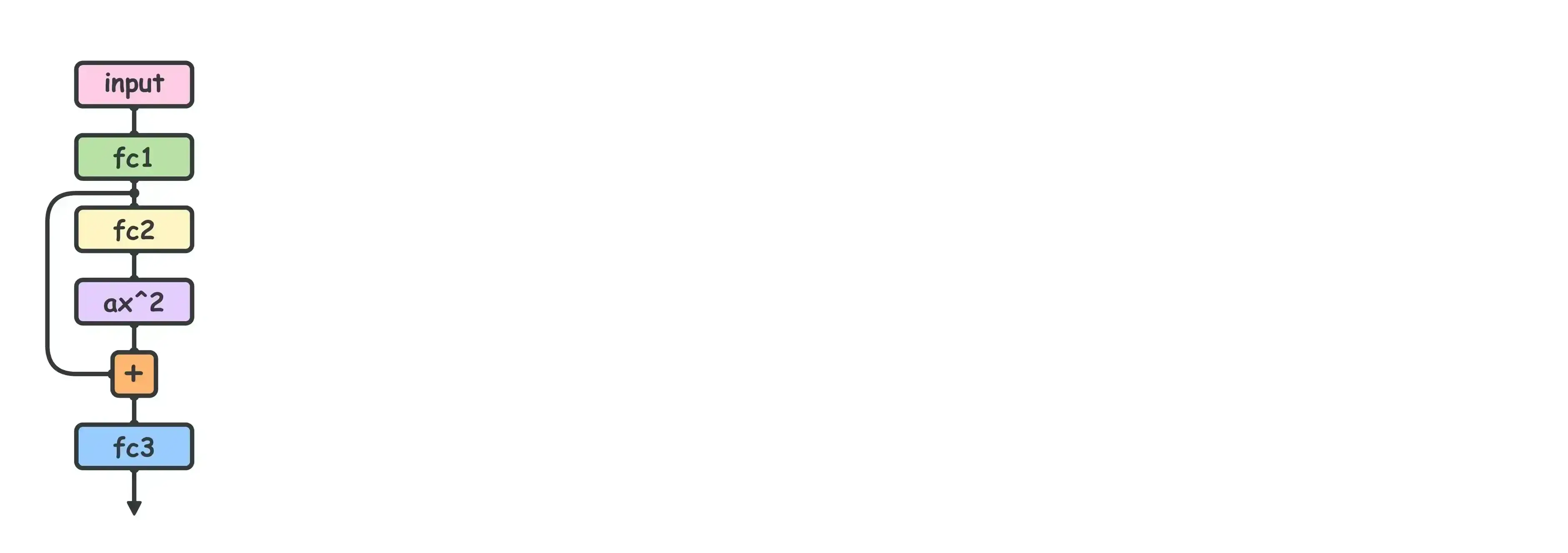
Figure 7 (left) visualizes this DAG for a simple 3-layer MLP without intermediate activation functions. Here, nodes within a row represent possible choices of level for each linear layer, weighted by the latency of performing that linear layer at the given level. Each row also excludes invalid states. For instance, there is no node for fc2 at level l=0 because linear layers consume a level, and we could lose decoding correctness if there were.

We can then weigh the edges between layers by whether a bootstrap operation is required. For instance, the edges highlighted in red in Figure 7 (middle) each increase the level of the ciphertext (after the layer itself is performed), and therefore must be bootstrapped.
With these two constraints, we can apply a shortest path algorithm to find the path that minimizes end-to-end latency in Figure 7 (right). With respect to our heuristics, this shortest path gives us both the optimal locations to bootstrap and the optimal levels at which to perform each layer.
4a. Beyond Simple MLPs
This method extends almost directly to more complex networks, especially those with residual connections. The main obstacle is that residual connections create multiple paths through the graph, each sharing a common fork and join node. This makes directly applying our shortest path approach challenging.
We solve this by creating two level DAGs around each residual connection: one for the backbone, one for the residual itself. Then, we can (i) sum the shortest paths for all possible pairs of input and output nodes, and (ii) insert that black-boxed solution back into the original level DAG. This reduces the problem to our original shortest path approach.
Interestingly, this approach extends recursively to graphs with any number of fork/join pairs. Figure 9 gives the high-level solution for attention blocks within transformers.

5. Addressing the Sharp Bits
There’s still more to running deep FHE inference beyond packing and bootstrap placement. Orion includes several automation layers that remove the “sharp edges” that typically trip up non-experts.
First, to conform to the CKKS programming model, all non-linear functions (e.g., ReLU or GELU) must be replaced by high-degree polynomials over the correct range. Orion automates this with orion.fit() which iterates over the training data and (i) replaces non-linearities with Chebyshev polynomials, and (ii) automatically determines the input ranges those approximations need.
Second, Orion automates scale management. We leverage the fact that our compilation phase has already determined the level at which to perform any linear layer (call it level $j$). We encode the weights with scale factor $q_j$ (the last RNS modulus at level $j$) rather than $\Delta$. This way, performing a convolution with a ciphertext at scale $\Delta$ produces an output at scale $\Delta \cdot q_j$. Rescaling divides by $q_j$, resetting the scale back to exactly $\Delta$. This is what we call “errorless” neural network evaluation.
Finally, Orion handles the large data structures that come with FHE inference. Server-side packed vectors and evaluation keys can reach tens to hundreds of gigabytes. Orion optionally reduces memory pressure by dynamically loading per-layer plaintext vectors during linear transforms.

From the user’s perspective, Orion feels like PyTorch: you write a model as usual, fit/compile it for FHE, and run encrypted inference.
Click to expand: Model definition (ResNet-20)
import torch.nn as nn
import orion.nn as on


class BasicBlock(on.Module):
    expansion = 1

    def __init__(self, Ci, Co, stride=1):
        super().__init__()
        self.conv1 = on.Conv2d(Ci, Co, kernel_size=3, stride=stride, padding=1, bias=False)
        self.bn1   = on.BatchNorm2d(Co)
        self.act1  = on.ReLU()

        self.conv2 = on.Conv2d(Co, Co, kernel_size=3, stride=1, padding=1, bias=False)
        self.bn2   = on.BatchNorm2d(Co)
        self.act2  = on.ReLU()

        self.add = on.Add()
        self.shortcut = nn.Sequential()
        if stride != 1 or Ci != self.expansion*Co:
            self.shortcut = nn.Sequential(
                on.Conv2d(Ci, self.expansion*Co, kernel_size=1, stride=stride, bias=False),
                on.BatchNorm2d(self.expansion*Co))

    def forward(self, x):
        out = self.act1(self.bn1(self.conv1(x)))
        out = self.bn2(self.conv2(out))
        out = self.add(out, self.shortcut(x))
        return self.act2(out)


class ResNet(on.Module):
    def __init__(self, dataset, block, num_blocks, num_chans, conv1_params, num_classes):
        super().__init__()
        self.in_chans = num_chans[0]
        self.last_chans = num_chans[-1]

        self.conv1 = on.Conv2d(3, self.in_chans, **conv1_params, bias=False)
        self.bn1 = on.BatchNorm2d(self.in_chans)
        self.act = on.ReLU()

        self.layers = nn.ModuleList()
        for i in range(len(num_blocks)):
            stride = 1 if i == 0 else 2
            self.layers.append(self.layer(block, num_chans[i], num_blocks[i], stride))

        self.avgpool = on.AdaptiveAvgPool2d(output_size=(1,1))
        self.flatten = on.Flatten()
        self.linear  = on.Linear(self.last_chans * block.expansion, num_classes)

    def layer(self, block, chans, num_blocks, stride):
        strides = [stride] + [1]*(num_blocks-1)
        layers = []
        for stride in strides:
            layers.append(block(self.in_chans, chans, stride))
            self.in_chans = chans * block.expansion
        return nn.Sequential(*layers)

    def forward(self, x):
        out = self.act(self.bn1(self.conv1(x)))
        for layer in self.layers:
            out = layer(out)

        out = self.avgpool(out)
        out = self.flatten(out)
        return self.linear(out)


def ResNet20(dataset='cifar10'):
    configs = {
        "cifar10":  {"kernel_size": 3, "stride": 1, "padding": 1, "num_classes": 10},
        "cifar100": {"kernel_size": 3, "stride": 1, "padding": 1, "num_classes": 100},
    }
    config = configs[dataset]
    conv1_params = {
        'kernel_size': config["kernel_size"],
        'stride': config["stride"],
        'padding': config["padding"]
    }
    return ResNet(dataset, BasicBlock, [3,3,3], [16,32,64], conv1_params, config["num_classes"])
Click to expand: FHE compilation workflow
# High-level workflow (sketch)
net = ResNet20()
orion.fit(net, trainloader)   # range discovery + polynomial activation replacement
orion.compile(net)            # packing + bootstrap placement + key/material generation

net.he()                      # switch model into FHE execution mode
ct_out = net(ct_in)           # run encrypted inference
6. Results
To highlight Orion’s scalability, we ran ResNet-34 and ResNet-50 on ImageNet end-to-end under FHE with single-threaded inference times of 3.98 hours and 8.98 hours, respectively. To show that Orion handles more than classification, we also ran object detection using a 139 million parameter YOLO-v1 model on the PASCAL-VOC dataset (images of size 448 $\times$ 448 $\times$ 3). An encrypted inference took 17.5 hours and produced bounding boxes and confidence scores entirely under FHE, matching the cleartext PyTorch output to 8 bits of precision.

If you want to reproduce results or try Orion on your own models, the repository is available at https://github.com/baahl-nyu/orion.
References
-
Eunsang Lee, Joon-Woo Lee, Junghyun Lee, Young-Sik Kim, Yongjune Kim, Jong-Seon No, and Woosuk Choi. “Low-Complexity Deep Convolutional Neural Networks on Fully Homomorphic Encryption Using Multiplexed Parallel Convolutions.” ICML 2022. https://proceedings.mlr.press/v162/lee22e.html ↩